Table of Contents:
- Transformers Overview
- Why Transformers?
- Multi-Headed Attention
- Multi-Headed Attention Tips
- Transformer Steps: Encoder-Decoder
Transformer Overview
In “Attention Is All You Need”, Vaswani et al. introduced the Transformer, which introduces parallelism and enables models to learn long-range dependencies–thereby helping solve two key issues with RNNs: their slow speed of training and their difficulty in encoding long-range dependencies. Transformers are highly scalable and highly parallelizable, allowing for faster training, larger models, and better performance across vision and language tasks. Transformers are beginning to replace RNNs and LSTMs and may soon replace convolutions as well.
Why Transformers?
- Transformers are great for working with long input sequences since the attention calculation looks at all inputs. In contrast, RNNs struggle to encode long-range dependencies. LSTMs are much better at capturing long-range dependencies by using the input, output, and forget gates.
- Transformers can operate over unordered sets or ordered sequences with positional encodings (using positional encoding to add ordering the sets). In contrast, RNN/LSTM expect an ordered sequence of inputs.
- Transformers use parallel computation where all alignment and attention scores for all inputs can be done in parallel. In contrast, RNN/LSTM uses sequential computation since the hidden state at a current timestep can only be computed after the previous states are calculated which makes them often slow to train.
Multi-Headed Attention
Let’s refresh our concepts from the attention unit to help us with transformers.
- Dot-Product Attention:

With query q (D,), value vectors {v_1,…,v_n} where v_i (D,), key vectors {k_1,…,k_n} where k_i (D,), attention weights a_i, and output c (D,).
The output is a weighted average over the value vectors.
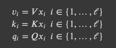
- Self-Attention: we derive values, keys, and queries from the input

Combining the above two, we can now implement multi-headed scaled dot product attention for transformers.
- Multi-Headed Scaled Dot Product Attention: We learn a parameter matrix V_i, K_i, Q_i (DxD) for each head i, which increases the model’s expressivity to attend to different parts of the input. We apply a scaling term (1/sqrt(d/h)) to the dot-product attention described previously in order to reduce the effect of large magnitude vectors.

We can then apply dropout, generate the output of the attention layer, and finally add a linear transformation to the output of the attention operation, which allows the model to learn the relationship between heads, thereby improving the model’s expressivity.
Step-by-Step Multi-Headed Attention with Intermediate Dimensions
There’s a lot happening throughout the Multi-Headed Attention so hopefully this chart will help further clarify the intermediate steps and how the dimensions change after each step!
A couple tips on Permute and Reshape:
To create the multiple heads, we divide the embedding dimension by the number of heads and use Reshape (Ex: Reshape allows us to go from shape (N x S x D) to (N x S x H x D//H) ). It is important to note that Reshape doesn’t change the ordering of your data. It simply takes the original data and ‘reshapes’ it into the dimensions you provide. We use Permute (or can use Transpose) to rearrange the ordering of dimensions of the data (Ex: Permute allows us to rearrange the dimensions from (N x S x H x D//H) to (N x H x S x D//H) ). Notice why we needed to use Permute before Reshaping after the final MatMul operation. Our current tensor had a shape of (N x H x S x D//H) but in order to reshape it to be (N x S x D) we needed to first ensure that the H and D//H dimensions are right next to each other because reshape doesn’t change the ordering of the data. Therefore we use Permute first to rearrange the dimensions from (N x H x S x D//H) to (N x S x H x D//H) and then can use reshape to get the shape of (N x S x D).
Transformer Steps: Encoder-Decoder
Encoder Block
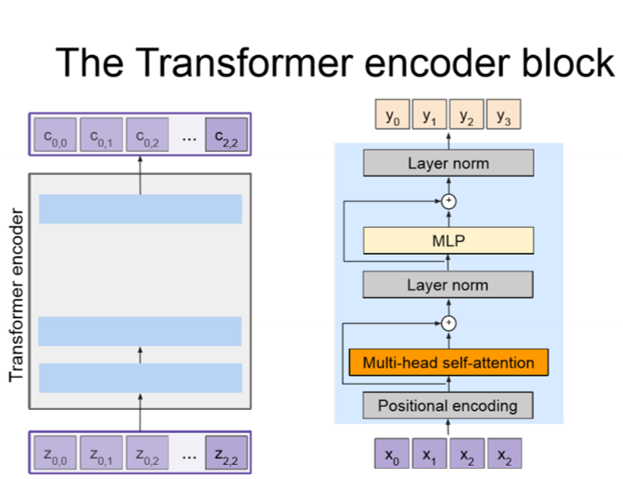
The role of the Encoder block is to encode all the image features (where the spatial features are extracted using pretrained CNN) into a set of context vectors. The context vectors outputted are a representation of the input sequence in a higher dimensional space. We define the Encoder as c = T_W(z) where z is the spatial CNN features and T_w(.) is the transformer encoder. In the “Attention Is All You Need” paper a transformer encoder block made up of N encoder blocks (N = 6, D = 512) is used.

Let’s walk through the steps of the Encoder block!
- We first take in a set of input vectors X (where each input vector represents a word for instance)
- We then add positional encoding to the input vectors.
- We pass the positional encoded vectors through the Multi-head self-attention layer (where each vector attends on all the other vectors). The output of this layer gives us a set of context vectors.
- We have a Residual Connection after the Multi-head self-attention layer which allows us to bypass the attention layer if it’s not needed.
- We then apply Layer Normalization on the output which normalizes each individual vector.
- We then apply MLP over each vector individually.
- We then have another Residual Connection.
- A final Layer Normalization on the output.
- And finally the set of context vectors C is outputted!
Decoder Block
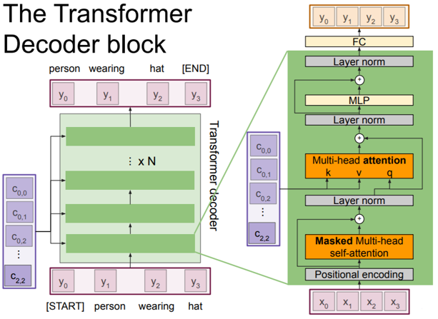
The Decoder block takes in the set of context vectors C outputted from the encoder block and set of input vectors X and outputs a set of vectors Y which defines the output sequence. We define the Decoder as y_t = T_S(y_{0:t-1},c) where T_D( .) is the transformer decoder. In the”Attention Is All You Need” paper a transformer decoder block made up of N decoder blocks (N = 6, D = 512) is used.

Let’s walk through the steps of the Decoder block!
- We take in the set of input vectors X and context vectors C (outputted from Encoder block)
- We then add positional encoding to the input vectors X.
- We pass the positional encoded vectors through the Masked Multi-head self-attention layer. The mask ensures that we only attend over previous inputs.
- We have a Residual Connection after this layer which allows us to bypass the attention layer if it’s not needed.
- We then apply Layer Normalization on the output which normalizes each individual vector.
- Then we pass the output through another Multi-head attention layer which takes in the context vectors outputted by the Encoder block as well as the output of the Layer Normalization. In this step the Key comes from the set of context vectors C, the Value comes from the set of context vectors C, and the Query comes from the output of the Layer Normalization step.
- We then have another Residual Connection.
- Apply another Layer Normalization.
- Apply MLP over each vector individually.
- Another Residual Connection
- A final Layer Normalization
- And finally we pass the output through a Fully-connected layer which produces the final set of output vectors Y which is the output sequence.
Additional Notes on Layer Normalization and MLP
Layer Normalization: As seen in the Encoder and Decoder block implementation, we use Layer Normalization after the Residual Connections in both the Encoder and Decoder Blocks. Recall that in Layer Normalization we are normalizing across the feature dimension (so we are applying LayerNorm over the image features). Using Layer Normalization at these points helps us prevent issues with vanishing or exploding gradients, helps stabilize the network, and can reduce training time.
MLP: Both the encoder and decoder blocks contain position-wise fully-connected feed-forward networks, which are “applied to each position separately and identically” (Vaswani et al.). The linear transformations use different parameters across layers. FFN(x) = max(0, xW_1 + b_1)W_2 + b_2. Additionally, the combination of a self-attention layer and a point-wise feed-forward layer reduces the complexity required by convolutional layers.
Additional Resources
Additional resources related to implementation: