Table of Contents:
- Quick intro without brain analogies
- Modeling one neuron
- Neural Network architectures
- Summary
- Additional references
Quick intro
It is possible to introduce neural networks without appealing to brain analogies. In the section on linear classification we computed scores for different visual categories given the image using the formula \( s = W x \), where \(W\) was a matrix and \(x\) was an input column vector containing all pixel data of the image. In the case of CIFAR-10, \(x\) is a [3072x1] column vector, and \(W\) is a [10x3072] matrix, so that the output scores is a vector of 10 class scores.
An example neural network would instead compute \( s = W_2 \max(0, W_1 x) \). Here, \(W_1\) could be, for example, a [100x3072] matrix transforming the image into a 100-dimensional intermediate vector. The function \(max(0,-) \) is a non-linearity that is applied elementwise. There are several choices we could make for the non-linearity (which we’ll study below), but this one is a common choice and simply thresholds all activations that are below zero to zero. Finally, the matrix \(W_2\) would then be of size [10x100], so that we again get 10 numbers out that we interpret as the class scores. Notice that the non-linearity is critical computationally - if we left it out, the two matrices could be collapsed to a single matrix, and therefore the predicted class scores would again be a linear function of the input. The non-linearity is where we get the wiggle. The parameters \(W_2, W_1\) are learned with stochastic gradient descent, and their gradients are derived with chain rule (and computed with backpropagation).
A three-layer neural network could analogously look like \( s = W_3 \max(0, W_2 \max(0, W_1 x)) \), where all of \(W_3, W_2, W_1\) are parameters to be learned. The sizes of the intermediate hidden vectors are hyperparameters of the network and we’ll see how we can set them later. Lets now look into how we can interpret these computations from the neuron/network perspective.
Modeling one neuron
The area of Neural Networks has originally been primarily inspired by the goal of modeling biological neural systems, but has since diverged and become a matter of engineering and achieving good results in Machine Learning tasks. Nonetheless, we begin our discussion with a very brief and high-level description of the biological system that a large portion of this area has been inspired by.
Biological motivation and connections
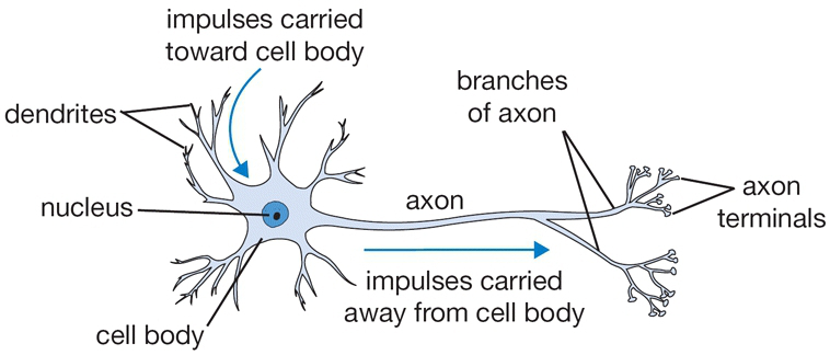
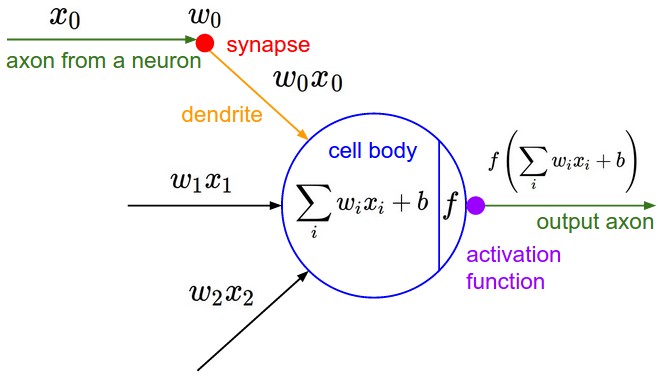
The basic computational unit of the brain is a neuron. Approximately 86 billion neurons can be found in the human nervous system and they are connected with approximately 10^14 - 10^15 synapses. The diagram below shows a cartoon drawing of a biological neuron (left) and a common mathematical model (right). Each neuron receives input signals from its dendrites and produces output signals along its (single) axon. The axon eventually branches out and connects via synapses to dendrites of other neurons. In the computational model of a neuron, the signals that travel along the axons (e.g. \(x_0\)) interact multiplicatively (e.g. \(w_0 x_0\)) with the dendrites of the other neuron based on the synaptic strength at that synapse (e.g. \(w_0\)). The idea is that the synaptic strengths (the weights \(w\)) are learnable and control the strength of influence (and its direction: excitory (positive weight) or inhibitory (negative weight)) of one neuron on another. In the basic model, the dendrites carry the signal to the cell body where they all get summed. If the final sum is above a certain threshold, the neuron can fire, sending a spike along its axon. In the computational model, we assume that the precise timings of the spikes do not matter, and that only the frequency of the firing communicates information. Based on this rate code interpretation, we model the firing rate of the neuron with an activation function \(f\), which represents the frequency of the spikes along the axon. Historically, a common choice of activation function is the sigmoid function \(\sigma\), since it takes a real-valued input (the signal strength after the sum) and squashes it to range between 0 and 1. We will see details of these activation functions later in this section.
An example code for forward-propagating a single neuron might look as follows:
class Neuron(object):
  # ...
  def forward(self, inputs):
    """ assume inputs and weights are 1-D numpy arrays and bias is a number """
    cell_body_sum = np.sum(inputs * self.weights) + self.bias
    firing_rate = 1.0 / (1.0 + math.exp(-cell_body_sum)) # sigmoid activation function
    return firing_rate
In other words, each neuron performs a dot product with the input and its weights, adds the bias and applies the non-linearity (or activation function), in this case the sigmoid \(\sigma(x) = 1/(1+e^{-x})\). We will go into more details about different activation functions at the end of this section.
Coarse model. It’s important to stress that this model of a biological neuron is very coarse: For example, there are many different types of neurons, each with different properties. The dendrites in biological neurons perform complex nonlinear computations. The synapses are not just a single weight, they’re a complex non-linear dynamical system. The exact timing of the output spikes in many systems is known to be important, suggesting that the rate code approximation may not hold. Due to all these and many other simplifications, be prepared to hear groaning sounds from anyone with some neuroscience background if you draw analogies between Neural Networks and real brains. See this review (pdf), or more recently this review if you are interested.
Single neuron as a linear classifier
The mathematical form of the model Neuron’s forward computation might look familiar to you. As we saw with linear classifiers, a neuron has the capacity to “like” (activation near one) or “dislike” (activation near zero) certain linear regions of its input space. Hence, with an appropriate loss function on the neuron’s output, we can turn a single neuron into a linear classifier:
Binary Softmax classifier. For example, we can interpret \(\sigma(\sum_iw_ix_i + b)\) to be the probability of one of the classes \(P(y_i = 1 \mid x_i; w) \). The probability of the other class would be \(P(y_i = 0 \mid x_i; w) = 1 - P(y_i = 1 \mid x_i; w) \), since they must sum to one. With this interpretation, we can formulate the cross-entropy loss as we have seen in the Linear Classification section, and optimizing it would lead to a binary Softmax classifier (also known as logistic regression). Since the sigmoid function is restricted to be between 0-1, the predictions of this classifier are based on whether the output of the neuron is greater than 0.5.
Binary SVM classifier. Alternatively, we could attach a max-margin hinge loss to the output of the neuron and train it to become a binary Support Vector Machine.
Regularization interpretation. The regularization loss in both SVM/Softmax cases could in this biological view be interpreted as gradual forgetting, since it would have the effect of driving all synaptic weights \(w\) towards zero after every parameter update.
A single neuron can be used to implement a binary classifier (e.g. binary Softmax or binary SVM classifiers)
Commonly used activation functions
Every activation function (or non-linearity) takes a single number and performs a certain fixed mathematical operation on it. There are several activation functions you may encounter in practice:
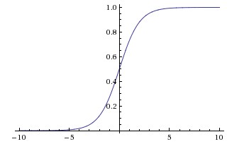
Sigmoid. The sigmoid non-linearity has the mathematical form \(\sigma(x) = 1 / (1 + e^{-x})\) and is shown in the image above on the left. As alluded to in the previous section, it takes a real-valued number and “squashes” it into range between 0 and 1. In particular, large negative numbers become 0 and large positive numbers become 1. The sigmoid function has seen frequent use historically since it has a nice interpretation as the firing rate of a neuron: from not firing at all (0) to fully-saturated firing at an assumed maximum frequency (1). In practice, the sigmoid non-linearity has recently fallen out of favor and it is rarely ever used. It has two major drawbacks:
- Sigmoids saturate and kill gradients. A very undesirable property of the sigmoid neuron is that when the neuron’s activation saturates at either tail of 0 or 1, the gradient at these regions is almost zero. Recall that during backpropagation, this (local) gradient will be multiplied to the gradient of this gate’s output for the whole objective. Therefore, if the local gradient is very small, it will effectively “kill” the gradient and almost no signal will flow through the neuron to its weights and recursively to its data. Additionally, one must pay extra caution when initializing the weights of sigmoid neurons to prevent saturation. For example, if the initial weights are too large then most neurons would become saturated and the network will barely learn.
- Sigmoid outputs are not zero-centered. This is undesirable since neurons in later layers of processing in a Neural Network (more on this soon) would be receiving data that is not zero-centered. This has implications on the dynamics during gradient descent, because if the data coming into a neuron is always positive (e.g. \(x > 0\) elementwise in \(f = w^Tx + b\))), then the gradient on the weights \(w\) will during backpropagation become either all be positive, or all negative (depending on the gradient of the whole expression \(f\)). This could introduce undesirable zig-zagging dynamics in the gradient updates for the weights. However, notice that once these gradients are added up across a batch of data the final update for the weights can have variable signs, somewhat mitigating this issue. Therefore, this is an inconvenience but it has less severe consequences compared to the saturated activation problem above.
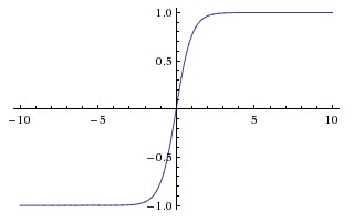
Tanh. The tanh non-linearity is shown on the image above on the right. It squashes a real-valued number to the range [-1, 1]. Like the sigmoid neuron, its activations saturate, but unlike the sigmoid neuron its output is zero-centered. Therefore, in practice the tanh non-linearity is always preferred to the sigmoid nonlinearity. Also note that the tanh neuron is simply a scaled sigmoid neuron, in particular the following holds: \( \tanh(x) = 2 \sigma(2x) -1 \).
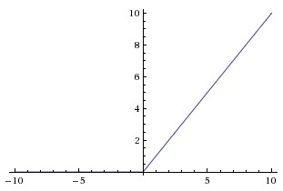
ReLU. The Rectified Linear Unit has become very popular in the last few years. It computes the function \(f(x) = \max(0, x)\). In other words, the activation is simply thresholded at zero (see image above on the left). There are several pros and cons to using the ReLUs:
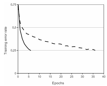
- (+) It was found to greatly accelerate (e.g. a factor of 6 in Krizhevsky et al.) the convergence of stochastic gradient descent compared to the sigmoid/tanh functions. It is argued that this is due to its linear, non-saturating form.
- (+) Compared to tanh/sigmoid neurons that involve expensive operations (exponentials, etc.), the ReLU can be implemented by simply thresholding a matrix of activations at zero.
- (-) Unfortunately, ReLU units can be fragile during training and can “die”. For example, a large gradient flowing through a ReLU neuron could cause the weights to update in such a way that the neuron will never activate on any datapoint again. If this happens, then the gradient flowing through the unit will forever be zero from that point on. That is, the ReLU units can irreversibly die during training since they can get knocked off the data manifold. For example, you may find that as much as 40% of your network can be “dead” (i.e. neurons that never activate across the entire training dataset) if the learning rate is set too high. With a proper setting of the learning rate this is less frequently an issue.
Leaky ReLU. Leaky ReLUs are one attempt to fix the “dying ReLU” problem. Instead of the function being zero when x < 0, a leaky ReLU will instead have a small positive slope (of 0.01, or so). That is, the function computes \(f(x) = \mathbb{1}(x < 0) (\alpha x) + \mathbb{1}(x>=0) (x) \) where \(\alpha\) is a small constant. Some people report success with this form of activation function, but the results are not always consistent. The slope in the negative region can also be made into a parameter of each neuron, as seen in PReLU neurons, introduced in Delving Deep into Rectifiers, by Kaiming He et al., 2015. However, the consistency of the benefit across tasks is presently unclear.
Maxout. Other types of units have been proposed that do not have the functional form \(f(w^Tx + b)\) where a non-linearity is applied on the dot product between the weights and the data. One relatively popular choice is the Maxout neuron (introduced recently by Goodfellow et al.) that generalizes the ReLU and its leaky version. The Maxout neuron computes the function \(\max(w_1^Tx+b_1, w_2^Tx + b_2)\). Notice that both ReLU and Leaky ReLU are a special case of this form (for example, for ReLU we have \(w_1, b_1 = 0\)). The Maxout neuron therefore enjoys all the benefits of a ReLU unit (linear regime of operation, no saturation) and does not have its drawbacks (dying ReLU). However, unlike the ReLU neurons it doubles the number of parameters for every single neuron, leading to a high total number of parameters.
This concludes our discussion of the most common types of neurons and their activation functions. As a last comment, it is very rare to mix and match different types of neurons in the same network, even though there is no fundamental problem with doing so.
TLDR: “What neuron type should I use?” Use the ReLU non-linearity, be careful with your learning rates and possibly monitor the fraction of “dead” units in a network. If this concerns you, give Leaky ReLU or Maxout a try. Never use sigmoid. Try tanh, but expect it to work worse than ReLU/Maxout.
Neural Network architectures
Layer-wise organization
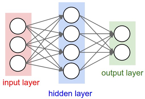
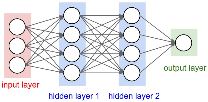
Neural Networks as neurons in graphs. Neural Networks are modeled as collections of neurons that are connected in an acyclic graph. In other words, the outputs of some neurons can become inputs to other neurons. Cycles are not allowed since that would imply an infinite loop in the forward pass of a network. Instead of an amorphous blobs of connected neurons, Neural Network models are often organized into distinct layers of neurons. For regular neural networks, the most common layer type is the fully-connected layer in which neurons between two adjacent layers are fully pairwise connected, but neurons within a single layer share no connections. Below are two example Neural Network topologies that use a stack of fully-connected layers:
Naming conventions. Notice that when we say N-layer neural network, we do not count the input layer. Therefore, a single-layer neural network describes a network with no hidden layers (input directly mapped to output). In that sense, you can sometimes hear people say that logistic regression or SVMs are simply a special case of single-layer Neural Networks. You may also hear these networks interchangeably referred to as “Artificial Neural Networks” (ANN) or “Multi-Layer Perceptrons” (MLP). Many people do not like the analogies between Neural Networks and real brains and prefer to refer to neurons as units.
Output layer. Unlike all layers in a Neural Network, the output layer neurons most commonly do not have an activation function (or you can think of them as having a linear identity activation function). This is because the last output layer is usually taken to represent the class scores (e.g. in classification), which are arbitrary real-valued numbers, or some kind of real-valued target (e.g. in regression).
Sizing neural networks. The two metrics that people commonly use to measure the size of neural networks are the number of neurons, or more commonly the number of parameters. Working with the two example networks in the above picture:
- The first network (left) has 4 + 2 = 6 neurons (not counting the inputs), [3 x 4] + [4 x 2] = 20 weights and 4 + 2 = 6 biases, for a total of 26 learnable parameters.
- The second network (right) has 4 + 4 + 1 = 9 neurons, [3 x 4] + [4 x 4] + [4 x 1] = 12 + 16 + 4 = 32 weights and 4 + 4 + 1 = 9 biases, for a total of 41 learnable parameters.
To give you some context, modern Convolutional Networks contain on orders of 100 million parameters and are usually made up of approximately 10-20 layers (hence deep learning). However, as we will see the number of effective connections is significantly greater due to parameter sharing. More on this in the Convolutional Neural Networks module.
Example feed-forward computation
Repeated matrix multiplications interwoven with activation function. One of the primary reasons that Neural Networks are organized into layers is that this structure makes it very simple and efficient to evaluate Neural Networks using matrix vector operations. Working with the example three-layer neural network in the diagram above, the input would be a [3x1] vector. All connection strengths for a layer can be stored in a single matrix. For example, the first hidden layer’s weights W1 would be of size [4x3], and the biases for all units would be in the vector b1, of size [4x1]. Here, every single neuron has its weights in a row of W1, so the matrix vector multiplication np.dot(W1,x) evaluates the activations of all neurons in that layer. Similarly, W2 would be a [4x4] matrix that stores the connections of the second hidden layer, and W3 a [1x4] matrix for the last (output) layer. The full forward pass of this 3-layer neural network is then simply three matrix multiplications, interwoven with the application of the activation function:
# forward-pass of a 3-layer neural network:
f = lambda x: 1.0/(1.0 + np.exp(-x)) # activation function (use sigmoid)
x = np.random.randn(3, 1) # random input vector of three numbers (3x1)
h1 = f(np.dot(W1, x) + b1) # calculate first hidden layer activations (4x1)
h2 = f(np.dot(W2, h1) + b2) # calculate second hidden layer activations (4x1)
out = np.dot(W3, h2) + b3 # output neuron (1x1)
In the above code, W1,W2,W3,b1,b2,b3 are the learnable parameters of the network. Notice also that instead of having a single input column vector, the variable x could hold an entire batch of training data (where each input example would be a column of x) and then all examples would be efficiently evaluated in parallel. Notice that the final Neural Network layer usually doesn’t have an activation function (e.g. it represents a (real-valued) class score in a classification setting).
The forward pass of a fully-connected layer corresponds to one matrix multiplication followed by a bias offset and an activation function.
Representational power
One way to look at Neural Networks with fully-connected layers is that they define a family of functions that are parameterized by the weights of the network. A natural question that arises is: What is the representational power of this family of functions? In particular, are there functions that cannot be modeled with a Neural Network?
It turns out that Neural Networks with at least one hidden layer are universal approximators. That is, it can be shown (e.g. see Approximation by Superpositions of Sigmoidal Function from 1989 (pdf), or this intuitive explanation from Michael Nielsen) that given any continuous function \(f(x)\) and some \(\epsilon > 0\), there exists a Neural Network \(g(x)\) with one hidden layer (with a reasonable choice of non-linearity, e.g. sigmoid) such that \( \forall x, \mid f(x) - g(x) \mid < \epsilon \). In other words, the neural network can approximate any continuous function.
If one hidden layer suffices to approximate any function, why use more layers and go deeper? The answer is that the fact that a two-layer Neural Network is a universal approximator is, while mathematically cute, a relatively weak and useless statement in practice. In one dimension, the “sum of indicator bumps” function \(g(x) = \sum_i c_i \mathbb{1}(a_i < x < b_i)\) where \(a,b,c\) are parameter vectors is also a universal approximator, but noone would suggest that we use this functional form in Machine Learning. Neural Networks work well in practice because they compactly express nice, smooth functions that fit well with the statistical properties of data we encounter in practice, and are also easy to learn using our optimization algorithms (e.g. gradient descent). Similarly, the fact that deeper networks (with multiple hidden layers) can work better than a single-hidden-layer networks is an empirical observation, despite the fact that their representational power is equal.
As an aside, in practice it is often the case that 3-layer neural networks will outperform 2-layer nets, but going even deeper (4,5,6-layer) rarely helps much more. This is in stark contrast to Convolutional Networks, where depth has been found to be an extremely important component for a good recognition system (e.g. on order of 10 learnable layers). One argument for this observation is that images contain hierarchical structure (e.g. faces are made up of eyes, which are made up of edges, etc.), so several layers of processing make intuitive sense for this data domain.
The full story is, of course, much more involved and a topic of much recent research. If you are interested in these topics we recommend for further reading:
- Deep Learning book in press by Bengio, Goodfellow, Courville, in particular Chapter 6.4.
- Do Deep Nets Really Need to be Deep?
- FitNets: Hints for Thin Deep Nets
Setting number of layers and their sizes
How do we decide on what architecture to use when faced with a practical problem? Should we use no hidden layers? One hidden layer? Two hidden layers? How large should each layer be? First, note that as we increase the size and number of layers in a Neural Network, the capacity of the network increases. That is, the space of representable functions grows since the neurons can collaborate to express many different functions. For example, suppose we had a binary classification problem in two dimensions. We could train three separate neural networks, each with one hidden layer of some size and obtain the following classifiers:
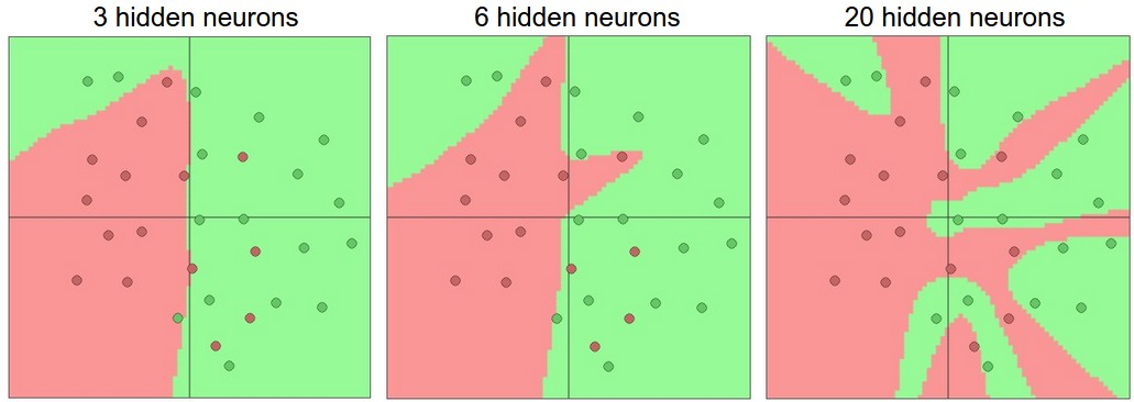
In the diagram above, we can see that Neural Networks with more neurons can express more complicated functions. However, this is both a blessing (since we can learn to classify more complicated data) and a curse (since it is easier to overfit the training data). Overfitting occurs when a model with high capacity fits the noise in the data instead of the (assumed) underlying relationship. For example, the model with 20 hidden neurons fits all the training data but at the cost of segmenting the space into many disjoint red and green decision regions. The model with 3 hidden neurons only has the representational power to classify the data in broad strokes. It models the data as two blobs and interprets the few red points inside the green cluster as outliers (noise). In practice, this could lead to better generalization on the test set.
Based on our discussion above, it seems that smaller neural networks can be preferred if the data is not complex enough to prevent overfitting. However, this is incorrect - there are many other preferred ways to prevent overfitting in Neural Networks that we will discuss later (such as L2 regularization, dropout, input noise). In practice, it is always better to use these methods to control overfitting instead of the number of neurons.
The subtle reason behind this is that smaller networks are harder to train with local methods such as Gradient Descent: It’s clear that their loss functions have relatively few local minima, but it turns out that many of these minima are easier to converge to, and that they are bad (i.e. with high loss). Conversely, bigger neural networks contain significantly more local minima, but these minima turn out to be much better in terms of their actual loss. Since Neural Networks are non-convex, it is hard to study these properties mathematically, but some attempts to understand these objective functions have been made, e.g. in a recent paper The Loss Surfaces of Multilayer Networks. In practice, what you find is that if you train a small network the final loss can display a good amount of variance - in some cases you get lucky and converge to a good place but in some cases you get trapped in one of the bad minima. On the other hand, if you train a large network you’ll start to find many different solutions, but the variance in the final achieved loss will be much smaller. In other words, all solutions are about equally as good, and rely less on the luck of random initialization.
To reiterate, the regularization strength is the preferred way to control the overfitting of a neural network. We can look at the results achieved by three different settings:
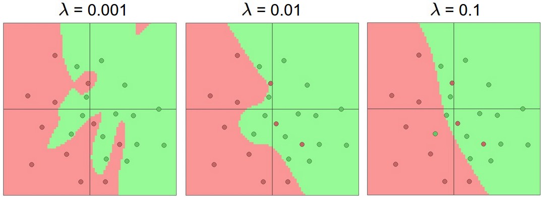
The takeaway is that you should not be using smaller networks because you are afraid of overfitting. Instead, you should use as big of a neural network as your computational budget allows, and use other regularization techniques to control overfitting.
Summary
In summary,
- We introduced a very coarse model of a biological neuron.
- We discussed several types of activation functions that are used in practice, with ReLU being the most common choice.
- We introduced Neural Networks where neurons are connected with Fully-Connected layers where neurons in adjacent layers have full pair-wise connections, but neurons within a layer are not connected.
- We saw that this layered architecture enables very efficient evaluation of Neural Networks based on matrix multiplications interwoven with the application of the activation function.
- We saw that that Neural Networks are universal function approximators, but we also discussed the fact that this property has little to do with their ubiquitous use. They are used because they make certain “right” assumptions about the functional forms of functions that come up in practice.
- We discussed the fact that larger networks will always work better than smaller networks, but their higher model capacity must be appropriately addressed with stronger regularization (such as higher weight decay), or they might overfit. We will see more forms of regularization (especially dropout) in later sections.
Additional References
- deeplearning.net tutorial with Theano
- ConvNetJS demos for intuitions
- Michael Nielsen’s tutorials