Table of Contents:
- Introduction
- Visualizing the loss function
- Optimization
- Computing the gradient
- Gradient descent
- Summary
Introduction
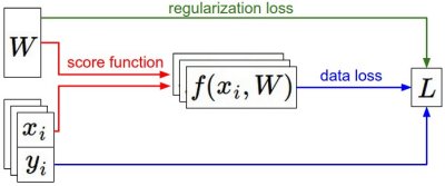
In the previous section we introduced two key components in context of the image classification task:
- A (parameterized) score function mapping the raw image pixels to class scores (e.g. a linear function)
- A loss function that measured the quality of a particular set of parameters based on how well the induced scores agreed with the ground truth labels in the training data. We saw that there are many ways and versions of this (e.g. Softmax/SVM).
Concretely, recall that the linear function had the form \( f(x_i, W) = W x_i \) and the SVM we developed was formulated as:
\[L = \frac{1}{N} \sum_i \sum_{j\neq y_i} \left[ \max(0, f(x_i; W)_j - f(x_i; W)_{y_i} + 1) \right] + \alpha R(W)\]We saw that a setting of the parameters \(W\) that produced predictions for examples \(x_i\) consistent with their ground truth labels \(y_i\) would also have a very low loss \(L\). We are now going to introduce the third and last key component: optimization. Optimization is the process of finding the set of parameters \(W\) that minimize the loss function.
Foreshadowing: Once we understand how these three core components interact, we will revisit the first component (the parameterized function mapping) and extend it to functions much more complicated than a linear mapping: First entire Neural Networks, and then Convolutional Neural Networks. The loss functions and the optimization process will remain relatively unchanged.
Visualizing the loss function
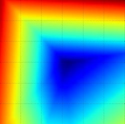
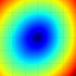
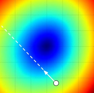
The loss functions we’ll look at in this class are usually defined over very high-dimensional spaces (e.g. in CIFAR-10 a linear classifier weight matrix is of size [10 x 3073] for a total of 30,730 parameters), making them difficult to visualize. However, we can still gain some intuitions about one by slicing through the high-dimensional space along rays (1 dimension), or along planes (2 dimensions). For example, we can generate a random weight matrix \(W\) (which corresponds to a single point in the space), then march along a ray and record the loss function value along the way. That is, we can generate a random direction \(W_1\) and compute the loss along this direction by evaluating \(L(W + a W_1)\) for different values of \(a\). This process generates a simple plot with the value of \(a\) as the x-axis and the value of the loss function as the y-axis. We can also carry out the same procedure with two dimensions by evaluating the loss \( L(W + a W_1 + b W_2) \) as we vary \(a, b\). In a plot, \(a, b\) could then correspond to the x-axis and the y-axis, and the value of the loss function can be visualized with a color:
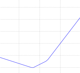
We can explain the piecewise-linear structure of the loss function by examining the math. For a single example we have:
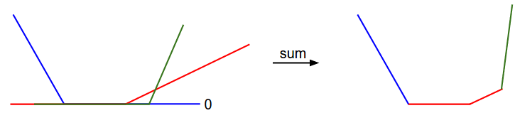
\[L_i = \sum_{j\neq y_i} \left[ \max(0, w_j^Tx_i - w_{y_i}^Tx_i + 1) \right]\]It is clear from the equation that the data loss for each example is a sum of (zero-thresholded due to the \(\max(0,-)\) function) linear functions of \(W\). Moreover, each row of \(W\) (i.e. \(w_j\)) sometimes has a positive sign in front of it (when it corresponds to a wrong class for an example), and sometimes a negative sign (when it corresponds to the correct class for that example). To make this more explicit, consider a simple dataset that contains three 1-dimensional points and three classes. The full SVM loss (without regularization) becomes:
\[\begin{align} L_0 = & \max(0, w_1^Tx_0 - w_0^Tx_0 + 1) + \max(0, w_2^Tx_0 - w_0^Tx_0 + 1) \\\\ L_1 = & \max(0, w_0^Tx_1 - w_1^Tx_1 + 1) + \max(0, w_2^Tx_1 - w_1^Tx_1 + 1) \\\\ L_2 = & \max(0, w_0^Tx_2 - w_2^Tx_2 + 1) + \max(0, w_1^Tx_2 - w_2^Tx_2 + 1) \\\\ L = & (L_0 + L_1 + L_2)/3 \end{align}\]Since these examples are 1-dimensional, the data \(x_i\) and weights \(w_j\) are numbers. Looking at, for instance, \(w_0\), some terms above are linear functions of \(w_0\) and each is clamped at zero. We can visualize this as follows:
As an aside, you may have guessed from its bowl-shaped appearance that the SVM cost function is an example of a convex function There is a large amount of literature devoted to efficiently minimizing these types of functions, and you can also take a Stanford class on the topic ( convex optimization ). Once we extend our score functions \(f\) to Neural Networks our objective functions will become non-convex, and the visualizations above will not feature bowls but complex, bumpy terrains.
Non-differentiable loss functions. As a technical note, you can also see that the kinks in the loss function (due to the max operation) technically make the loss function non-differentiable because at these kinks the gradient is not defined. However, the subgradient still exists and is commonly used instead. In this class will use the terms subgradient and gradient interchangeably.
Optimization
To reiterate, the loss function lets us quantify the quality of any particular set of weights W. The goal of optimization is to find W that minimizes the loss function. We will now motivate and slowly develop an approach to optimizing the loss function. For those of you coming to this class with previous experience, this section might seem odd since the working example we’ll use (the SVM loss) is a convex problem, but keep in mind that our goal is to eventually optimize Neural Networks where we can’t easily use any of the tools developed in the Convex Optimization literature.
Strategy #1: A first very bad idea solution: Random search
Since it is so simple to check how good a given set of parameters W is, the first (very bad) idea that may come to mind is to simply try out many different random weights and keep track of what works best. This procedure might look as follows:
# assume X_train is the data where each column is an example (e.g. 3073 x 50,000)
# assume Y_train are the labels (e.g. 1D array of 50,000)
# assume the function L evaluates the loss function

bestloss = float("inf") # Python assigns the highest possible float value
for num in range(1000):
  W = np.random.randn(10, 3073) * 0.0001 # generate random parameters
  loss = L(X_train, Y_train, W) # get the loss over the entire training set
  if loss < bestloss: # keep track of the best solution
    bestloss = loss
    bestW = W
  print 'in attempt %d the loss was %f, best %f' % (num, loss, bestloss)

# prints:
# in attempt 0 the loss was 9.401632, best 9.401632
# in attempt 1 the loss was 8.959668, best 8.959668
# in attempt 2 the loss was 9.044034, best 8.959668
# in attempt 3 the loss was 9.278948, best 8.959668
# in attempt 4 the loss was 8.857370, best 8.857370
# in attempt 5 the loss was 8.943151, best 8.857370
# in attempt 6 the loss was 8.605604, best 8.605604
# ... (trunctated: continues for 1000 lines)
In the code above, we see that we tried out several random weight vectors W, and some of them work better than others. We can take the best weights W found by this search and try it out on the test set:
# Assume X_test is [3073 x 10000], Y_test [10000 x 1]
scores = Wbest.dot(Xte_cols) # 10 x 10000, the class scores for all test examples
# find the index with max score in each column (the predicted class)
Yte_predict = np.argmax(scores, axis = 0)
# and calculate accuracy (fraction of predictions that are correct)
np.mean(Yte_predict == Yte)
# returns 0.1555
With the best W this gives an accuracy of about 15.5%. Given that guessing classes completely at random achieves only 10%, that’s not a very bad outcome for a such a brain-dead random search solution!
Core idea: iterative refinement. Of course, it turns out that we can do much better. The core idea is that finding the best set of weights W is a very difficult or even impossible problem (especially once W contains weights for entire complex neural networks), but the problem of refining a specific set of weights W to be slightly better is significantly less difficult. In other words, our approach will be to start with a random W and then iteratively refine it, making it slightly better each time.
Our strategy will be to start with random weights and iteratively refine them over time to get lower loss
Blindfolded hiker analogy. One analogy that you may find helpful going forward is to think of yourself as hiking on a hilly terrain with a blindfold on, and trying to reach the bottom. In the example of CIFAR-10, the hills are 30,730-dimensional, since the dimensions of W are 10 x 3073. At every point on the hill we achieve a particular loss (the height of the terrain).
Strategy #2: Random Local Search
The first strategy you may think of is to try to extend one foot in a random direction and then take a step only if it leads downhill. Concretely, we will start out with a random \(W\), generate random perturbations \( \delta W \) to it and if the loss at the perturbed \(W + \delta W\) is lower, we will perform an update. The code for this procedure is as follows:
W = np.random.randn(10, 3073) * 0.001 # generate random starting W
bestloss = float("inf")
for i in range(1000):
  step_size = 0.0001
  Wtry = W + np.random.randn(10, 3073) * step_size
  loss = L(Xtr_cols, Ytr, Wtry)
  if loss < bestloss:
    W = Wtry
    bestloss = loss
  print 'iter %d loss is %f' % (i, bestloss)
Using the same number of loss function evaluations as before (1000), this approach achieves test set classification accuracy of 21.4%. This is better, but still wasteful and computationally expensive.
Strategy #3: Following the Gradient
In the previous section we tried to find a direction in the weight-space that would improve our weight vector (and give us a lower loss). It turns out that there is no need to randomly search for a good direction: we can compute the best direction along which we should change our weight vector that is mathematically guaranteed to be the direction of the steepest descent (at least in the limit as the step size goes towards zero). This direction will be related to the gradient of the loss function. In our hiking analogy, this approach roughly corresponds to feeling the slope of the hill below our feet and stepping down the direction that feels steepest.
In one-dimensional functions, the slope is the instantaneous rate of change of the function at any point you might be interested in. The gradient is a generalization of slope for functions that don’t take a single number but a vector of numbers. Additionally, the gradient is just a vector of slopes (more commonly referred to as derivatives) for each dimension in the input space. The mathematical expression for the derivative of a 1-D function with respect its input is:
\[\frac{df(x)}{dx} = \lim_{h\ \to 0} \frac{f(x + h) - f(x)}{h}\]When the functions of interest take a vector of numbers instead of a single number, we call the derivatives partial derivatives, and the gradient is simply the vector of partial derivatives in each dimension.
Computing the gradient
There are two ways to compute the gradient: A slow, approximate but easy way (numerical gradient), and a fast, exact but more error-prone way that requires calculus (analytic gradient). We will now present both.
Computing the gradient numerically with finite differences
The formula given above allows us to compute the gradient numerically. Here is a generic function that takes a function f, a vector x to evaluate the gradient on, and returns the gradient of f at x:
def eval_numerical_gradient(f, x):
  """
  a naive implementation of numerical gradient of f at x
  - f should be a function that takes a single argument
  - x is the point (numpy array) to evaluate the gradient at
  """

  fx = f(x) # evaluate function value at original point
  grad = np.zeros(x.shape)
  h = 0.00001

  # iterate over all indexes in x
  it = np.nditer(x, flags=['multi_index'], op_flags=['readwrite'])
  while not it.finished:

    # evaluate function at x+h
    ix = it.multi_index
    old_value = x[ix]
    x[ix] = old_value + h # increment by h
    fxh = f(x) # evalute f(x + h)
    x[ix] = old_value # restore to previous value (very important!)

    # compute the partial derivative
    grad[ix] = (fxh - fx) / h # the slope
    it.iternext() # step to next dimension

  return grad
Following the gradient formula we gave above, the code above iterates over all dimensions one by one, makes a small change h along that dimension and calculates the partial derivative of the loss function along that dimension by seeing how much the function changed. The variable grad holds the full gradient in the end.
Practical considerations. Note that in the mathematical formulation the gradient is defined in the limit as h goes towards zero, but in practice it is often sufficient to use a very small value (such as 1e-5 as seen in the example). Ideally, you want to use the smallest step size that does not lead to numerical issues. Additionally, in practice it often works better to compute the numeric gradient using the centered difference formula: \( [f(x+h) - f(x-h)] / 2 h \) . See wiki for details.
We can use the function given above to compute the gradient at any point and for any function. Lets compute the gradient for the CIFAR-10 loss function at some random point in the weight space:
# to use the generic code above we want a function that takes a single argument
# (the weights in our case) so we close over X_train and Y_train
def CIFAR10_loss_fun(W):
  return L(X_train, Y_train, W)

W = np.random.rand(10, 3073) * 0.001 # random weight vector
df = eval_numerical_gradient(CIFAR10_loss_fun, W) # get the gradient
The gradient tells us the slope of the loss function along every dimension, which we can use to make an update:
loss_original = CIFAR10_loss_fun(W) # the original loss
print 'original loss: %f' % (loss_original, )

# lets see the effect of multiple step sizes
for step_size_log in [-10, -9, -8, -7, -6, -5,-4,-3,-2,-1]:
  step_size = 10 ** step_size_log
  W_new = W - step_size * df # new position in the weight space
  loss_new = CIFAR10_loss_fun(W_new)
  print 'for step size %f new loss: %f' % (step_size, loss_new)

# prints:
# original loss: 2.200718
# for step size 1.000000e-10 new loss: 2.200652
# for step size 1.000000e-09 new loss: 2.200057
# for step size 1.000000e-08 new loss: 2.194116
# for step size 1.000000e-07 new loss: 2.135493
# for step size 1.000000e-06 new loss: 1.647802
# for step size 1.000000e-05 new loss: 2.844355
# for step size 1.000000e-04 new loss: 25.558142
# for step size 1.000000e-03 new loss: 254.086573
# for step size 1.000000e-02 new loss: 2539.370888
# for step size 1.000000e-01 new loss: 25392.214036
Update in negative gradient direction. In the code above, notice that to compute W_new we are making an update in the negative direction of the gradient df since we wish our loss function to decrease, not increase.
Effect of step size. The gradient tells us the direction in which the function has the steepest rate of increase, but it does not tell us how far along this direction we should step. As we will see later in the course, choosing the step size (also called the learning rate) will become one of the most important (and most headache-inducing) hyperparameter settings in training a neural network. In our blindfolded hill-descent analogy, we feel the hill below our feet sloping in some direction, but the step length we should take is uncertain. If we shuffle our feet carefully we can expect to make consistent but very small progress (this corresponds to having a small step size). Conversely, we can choose to make a large, confident step in an attempt to descend faster, but this may not pay off. As you can see in the code example above, at some point taking a bigger step gives a higher loss as we “overstep”.
A problem of efficiency. You may have noticed that evaluating the numerical gradient has complexity linear in the number of parameters. In our example we had 30730 parameters in total and therefore had to perform 30,731 evaluations of the loss function to evaluate the gradient and to perform only a single parameter update. This problem only gets worse, since modern Neural Networks can easily have tens of millions of parameters. Clearly, this strategy is not scalable and we need something better.
Computing the gradient analytically with Calculus
The numerical gradient is very simple to compute using the finite difference approximation, but the downside is that it is approximate (since we have to pick a small value of h, while the true gradient is defined as the limit as h goes to zero), and that it is very computationally expensive to compute. The second way to compute the gradient is analytically using Calculus, which allows us to derive a direct formula for the gradient (no approximations) that is also very fast to compute. However, unlike the numerical gradient it can be more error prone to implement, which is why in practice it is very common to compute the analytic gradient and compare it to the numerical gradient to check the correctness of your implementation. This is called a gradient check.
Lets use the example of the SVM loss function for a single datapoint:
\[L_i = \sum_{j\neq y_i} \left[ \max(0, w_j^Tx_i - w_{y_i}^Tx_i + \Delta) \right]\]We can differentiate the function with respect to the weights. For example, taking the gradient with respect to \(w_{y_i}\) we obtain:
\[\nabla_{w_{y_i}} L_i = - \left( \sum_{j\neq y_i} \mathbb{1}(w_j^Tx_i - w_{y_i}^Tx_i + \Delta > 0) \right) x_i\]where \(\mathbb{1}\) is the indicator function that is one if the condition inside is true or zero otherwise. While the expression may look scary when it is written out, when you’re implementing this in code you’d simply count the number of classes that didn’t meet the desired margin (and hence contributed to the loss function) and then the data vector \(x_i\) scaled by this number is the gradient. Notice that this is the gradient only with respect to the row of \(W\) that corresponds to the correct class. For the other rows where \(j \neq y_i \) the gradient is:
\[\nabla_{w_j} L_i = \mathbb{1}(w_j^Tx_i - w_{y_i}^Tx_i + \Delta > 0) x_i\]Once you derive the expression for the gradient it is straight-forward to implement the expressions and use them to perform the gradient update.
Gradient Descent
Now that we can compute the gradient of the loss function, the procedure of repeatedly evaluating the gradient and then performing a parameter update is called Gradient Descent. Its vanilla version looks as follows:
# Vanilla Gradient Descent

while True:
  weights_grad = evaluate_gradient(loss_fun, data, weights)
  weights += - step_size * weights_grad # perform parameter update
This simple loop is at the core of all Neural Network libraries. There are other ways of performing the optimization (e.g. LBFGS), but Gradient Descent is currently by far the most common and established way of optimizing Neural Network loss functions. Throughout the class we will put some bells and whistles on the details of this loop (e.g. the exact details of the update equation), but the core idea of following the gradient until we’re happy with the results will remain the same.
Mini-batch gradient descent. In large-scale applications (such as the ILSVRC challenge), the training data can have on order of millions of examples. Hence, it seems wasteful to compute the full loss function over the entire training set in order to perform only a single parameter update. A very common approach to addressing this challenge is to compute the gradient over batches of the training data. For example, in current state of the art ConvNets, a typical batch contains 256 examples from the entire training set of 1.2 million. This batch is then used to perform a parameter update:
# Vanilla Minibatch Gradient Descent

while True:
  data_batch = sample_training_data(data, 256) # sample 256 examples
  weights_grad = evaluate_gradient(loss_fun, data_batch, weights)
  weights += - step_size * weights_grad # perform parameter update
The reason this works well is that the examples in the training data are correlated. To see this, consider the extreme case where all 1.2 million images in ILSVRC are in fact made up of exact duplicates of only 1000 unique images (one for each class, or in other words 1200 identical copies of each image). Then it is clear that the gradients we would compute for all 1200 identical copies would all be the same, and when we average the data loss over all 1.2 million images we would get the exact same loss as if we only evaluated on a small subset of 1000. In practice of course, the dataset would not contain duplicate images, the gradient from a mini-batch is a good approximation of the gradient of the full objective. Therefore, much faster convergence can be achieved in practice by evaluating the mini-batch gradients to perform more frequent parameter updates.
The extreme case of this is a setting where the mini-batch contains only a single example. This process is called Stochastic Gradient Descent (SGD) (or also sometimes on-line gradient descent). This is relatively less common to see because in practice due to vectorized code optimizations it can be computationally much more efficient to evaluate the gradient for 100 examples, than the gradient for one example 100 times. Even though SGD technically refers to using a single example at a time to evaluate the gradient, you will hear people use the term SGD even when referring to mini-batch gradient descent (i.e. mentions of MGD for “Minibatch Gradient Descent”, or BGD for “Batch gradient descent” are rare to see), where it is usually assumed that mini-batches are used. The size of the mini-batch is a hyperparameter but it is not very common to cross-validate it. It is usually based on memory constraints (if any), or set to some value, e.g. 32, 64 or 128. We use powers of 2 in practice because many vectorized operation implementations work faster when their inputs are sized in powers of 2.
Summary
In this section,
- We developed the intuition of the loss function as a high-dimensional optimization landscape in which we are trying to reach the bottom. The working analogy we developed was that of a blindfolded hiker who wishes to reach the bottom. In particular, we saw that the SVM cost function is piece-wise linear and bowl-shaped.
- We motivated the idea of optimizing the loss function with iterative refinement, where we start with a random set of weights and refine them step by step until the loss is minimized.
- We saw that the gradient of a function gives the steepest ascent direction and we discussed a simple but inefficient way of computing it numerically using the finite difference approximation (the finite difference being the value of h used in computing the numerical gradient).
- We saw that the parameter update requires a tricky setting of the step size (or the learning rate) that must be set just right: if it is too low the progress is steady but slow. If it is too high the progress can be faster, but more risky. We will explore this tradeoff in much more detail in future sections.
- We discussed the tradeoffs between computing the numerical and analytic gradient. The numerical gradient is simple but it is approximate and expensive to compute. The analytic gradient is exact, fast to compute but more error-prone since it requires the derivation of the gradient with math. Hence, in practice we always use the analytic gradient and then perform a gradient check, in which its implementation is compared to the numerical gradient.
- We introduced the Gradient Descent algorithm which iteratively computes the gradient and performs a parameter update in loop.
Coming up: The core takeaway from this section is that the ability to compute the gradient of a loss function with respect to its weights (and have some intuitive understanding of it) is the most important skill needed to design, train and understand neural networks. In the next section we will develop proficiency in computing the gradient analytically using the chain rule, otherwise also referred to as backpropagation. This will allow us to efficiently optimize relatively arbitrary loss functions that express all kinds of Neural Networks, including Convolutional Neural Networks.