Table of Contents:
- Gradient checks
- Sanity checks
- Babysitting the learning process
- Parameter updates
- Hyperparameter Optimization
- Evaluation
- Summary
- Additional References
Learning
In the previous sections we’ve discussed the static parts of a Neural Networks: how we can set up the network connectivity, the data, and the loss function. This section is devoted to the dynamics, or in other words, the process of learning the parameters and finding good hyperparameters.
Gradient Checks
In theory, performing a gradient check is as simple as comparing the analytic gradient to the numerical gradient. In practice, the process is much more involved and error prone. Here are some tips, tricks, and issues to watch out for:
Use the centered formula. The formula you may have seen for the finite difference approximation when evaluating the numerical gradient looks as follows:
\[\frac{df(x)}{dx} = \frac{f(x + h) - f(x)}{h} \hspace{0.1in} \text{(bad, do not use)}\]where \(h\) is a very small number, in practice approximately 1e-5 or so. In practice, it turns out that it is much better to use the centered difference formula of the form:
\[\frac{df(x)}{dx} = \frac{f(x + h) - f(x - h)}{2h} \hspace{0.1in} \text{(use instead)}\]This requires you to evaluate the loss function twice to check every single dimension of the gradient (so it is about 2 times as expensive), but the gradient approximation turns out to be much more precise. To see this, you can use Taylor expansion of \(f(x+h)\) and \(f(x-h)\) and verify that the first formula has an error on order of \(O(h)\), while the second formula only has error terms on order of \(O(h^2)\) (i.e. it is a second order approximation).
Use relative error for the comparison. What are the details of comparing the numerical gradient \(f’_n\) and analytic gradient \(f’_a\)? That is, how do we know if the two are not compatible? You might be temped to keep track of the difference \(\mid f’_a - f’_n \mid \) or its square and define the gradient check as failed if that difference is above a threshold. However, this is problematic. For example, consider the case where their difference is 1e-4. This seems like a very appropriate difference if the two gradients are about 1.0, so we’d consider the two gradients to match. But if the gradients were both on order of 1e-5 or lower, then we’d consider 1e-4 to be a huge difference and likely a failure. Hence, it is always more appropriate to consider the relative error:
\[\frac{\mid f'_a - f'_n \mid}{\max(\mid f'_a \mid, \mid f'_n \mid)}\]which considers their ratio of the differences to the ratio of the absolute values of both gradients. Notice that normally the relative error formula only includes one of the two terms (either one), but I prefer to max (or add) both to make it symmetric and to prevent dividing by zero in the case where one of the two is zero (which can often happen, especially with ReLUs). However, one must explicitly keep track of the case where both are zero and pass the gradient check in that edge case. In practice:
- relative error > 1e-2 usually means the gradient is probably wrong
- 1e-2 > relative error > 1e-4 should make you feel uncomfortable
- 1e-4 > relative error is usually okay for objectives with kinks. But if there are no kinks (e.g. use of tanh nonlinearities and softmax), then 1e-4 is too high.
- 1e-7 and less you should be happy.
Also keep in mind that the deeper the network, the higher the relative errors will be. So if you are gradient checking the input data for a 10-layer network, a relative error of 1e-2 might be okay because the errors build up on the way. Conversely, an error of 1e-2 for a single differentiable function likely indicates incorrect gradient.
Use double precision. A common pitfall is using single precision floating point to compute gradient check. It is often that case that you might get high relative errors (as high as 1e-2) even with a correct gradient implementation. In my experience I’ve sometimes seen my relative errors plummet from 1e-2 to 1e-8 by switching to double precision.
Stick around active range of floating point. It’s a good idea to read through “What Every Computer Scientist Should Know About Floating-Point Arithmetic”, as it may demystify your errors and enable you to write more careful code. For example, in neural nets it can be common to normalize the loss function over the batch. However, if your gradients per datapoint are very small, then additionally dividing them by the number of data points is starting to give very small numbers, which in turn will lead to more numerical issues. This is why I like to always print the raw numerical/analytic gradient, and make sure that the numbers you are comparing are not extremely small (e.g. roughly 1e-10 and smaller in absolute value is worrying). If they are you may want to temporarily scale your loss function up by a constant to bring them to a “nicer” range where floats are more dense - ideally on the order of 1.0, where your float exponent is 0.
Kinks in the objective. One source of inaccuracy to be aware of during gradient checking is the problem of kinks. Kinks refer to non-differentiable parts of an objective function, introduced by functions such as ReLU (\(max(0,x)\)), or the SVM loss, Maxout neurons, etc. Consider gradient checking the ReLU function at \(x = -1e6\). Since \(x < 0\), the analytic gradient at this point is exactly zero. However, the numerical gradient would suddenly compute a non-zero gradient because \(f(x+h)\) might cross over the kink (e.g. if \(h > 1e-6\)) and introduce a non-zero contribution. You might think that this is a pathological case, but in fact this case can be very common. For example, an SVM for CIFAR-10 contains up to 450,000 \(max(0,x)\) terms because there are 50,000 examples and each example yields 9 terms to the objective. Moreover, a Neural Network with an SVM classifier will contain many more kinks due to ReLUs.
Note that it is possible to know if a kink was crossed in the evaluation of the loss. This can be done by keeping track of the identities of all “winners” in a function of form \(max(x,y)\); That is, was x or y higher during the forward pass. If the identity of at least one winner changes when evaluating \(f(x+h)\) and then \(f(x-h)\), then a kink was crossed and the numerical gradient will not be exact.
Use only few datapoints. One fix to the above problem of kinks is to use fewer datapoints, since loss functions that contain kinks (e.g. due to use of ReLUs or margin losses etc.) will have fewer kinks with fewer datapoints, so it is less likely for you to cross one when you perform the finite different approximation. Moreover, if your gradcheck for only ~2 or 3 datapoints then you would almost certainly gradcheck for an entire batch. Using very few datapoints also makes your gradient check faster and more efficient.
Be careful with the step size h. It is not necessarily the case that smaller is better, because when \(h\) is much smaller, you may start running into numerical precision problems. Sometimes when the gradient doesn’t check, it is possible that you change \(h\) to be 1e-4 or 1e-6 and suddenly the gradient will be correct. This wikipedia article contains a chart that plots the value of h on the x-axis and the numerical gradient error on the y-axis.
Gradcheck during a “characteristic” mode of operation. It is important to realize that a gradient check is performed at a particular (and usually random), single point in the space of parameters. Even if the gradient check succeeds at that point, it is not immediately certain that the gradient is correctly implemented globally. Additionally, a random initialization might not be the most “characteristic” point in the space of parameters and may in fact introduce pathological situations where the gradient seems to be correctly implemented but isn’t. For instance, an SVM with very small weight initialization will assign almost exactly zero scores to all datapoints and the gradients will exhibit a particular pattern across all datapoints. An incorrect implementation of the gradient could still produce this pattern and not generalize to a more characteristic mode of operation where some scores are larger than others. Therefore, to be safe it is best to use a short burn-in time during which the network is allowed to learn and perform the gradient check after the loss starts to go down. The danger of performing it at the first iteration is that this could introduce pathological edge cases and mask an incorrect implementation of the gradient.
Don’t let the regularization overwhelm the data. It is often the case that a loss function is a sum of the data loss and the regularization loss (e.g. L2 penalty on weights). One danger to be aware of is that the regularization loss may overwhelm the data loss, in which case the gradients will be primarily coming from the regularization term (which usually has a much simpler gradient expression). This can mask an incorrect implementation of the data loss gradient. Therefore, it is recommended to turn off regularization and check the data loss alone first, and then the regularization term second and independently. One way to perform the latter is to hack the code to remove the data loss contribution. Another way is to increase the regularization strength so as to ensure that its effect is non-negligible in the gradient check, and that an incorrect implementation would be spotted.
Remember to turn off dropout/augmentations. When performing gradient check, remember to turn off any non-deterministic effects in the network, such as dropout, random data augmentations, etc. Otherwise these can clearly introduce huge errors when estimating the numerical gradient. The downside of turning off these effects is that you wouldn’t be gradient checking them (e.g. it might be that dropout isn’t backpropagated correctly). Therefore, a better solution might be to force a particular random seed before evaluating both \(f(x+h)\) and \(f(x-h)\), and when evaluating the analytic gradient.
Check only few dimensions. In practice the gradients can have sizes of million parameters. In these cases it is only practical to check some of the dimensions of the gradient and assume that the others are correct. Be careful: One issue to be careful with is to make sure to gradient check a few dimensions for every separate parameter. In some applications, people combine the parameters into a single large parameter vector for convenience. In these cases, for example, the biases could only take up a tiny number of parameters from the whole vector, so it is important to not sample at random but to take this into account and check that all parameters receive the correct gradients.
Before learning: sanity checks Tips/Tricks
Here are a few sanity checks you might consider running before you plunge into expensive optimization:
- Look for correct loss at chance performance. Make sure you’re getting the loss you expect when you initialize with small parameters. It’s best to first check the data loss alone (so set regularization strength to zero). For example, for CIFAR-10 with a Softmax classifier we would expect the initial loss to be 2.302, because we expect a diffuse probability of 0.1 for each class (since there are 10 classes), and Softmax loss is the negative log probability of the correct class so: -ln(0.1) = 2.302. For The Weston Watkins SVM, we expect all desired margins to be violated (since all scores are approximately zero), and hence expect a loss of 9 (since margin is 1 for each wrong class). If you’re not seeing these losses there might be issue with initialization.
- As a second sanity check, increasing the regularization strength should increase the loss
- Overfit a tiny subset of data. Lastly and most importantly, before training on the full dataset try to train on a tiny portion (e.g. 20 examples) of your data and make sure you can achieve zero cost. For this experiment it’s also best to set regularization to zero, otherwise this can prevent you from getting zero cost. Unless you pass this sanity check with a small dataset it is not worth proceeding to the full dataset. Note that it may happen that you can overfit very small dataset but still have an incorrect implementation. For instance, if your datapoints’ features are random due to some bug, then it will be possible to overfit your small training set but you will never notice any generalization when you fold it your full dataset.
Babysitting the learning process
There are multiple useful quantities you should monitor during training of a neural network. These plots are the window into the training process and should be utilized to get intuitions about different hyperparameter settings and how they should be changed for more efficient learning.
The x-axis of the plots below are always in units of epochs, which measure how many times every example has been seen during training in expectation (e.g. one epoch means that every example has been seen once). It is preferable to track epochs rather than iterations since the number of iterations depends on the arbitrary setting of batch size.
Loss function
The first quantity that is useful to track during training is the loss, as it is evaluated on the individual batches during the forward pass. Below is a cartoon diagram showing the loss over time, and especially what the shape might tell you about the learning rate:
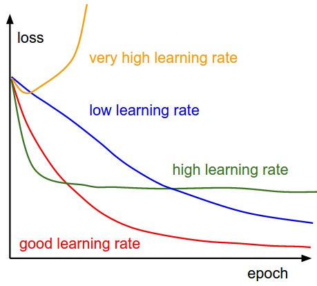
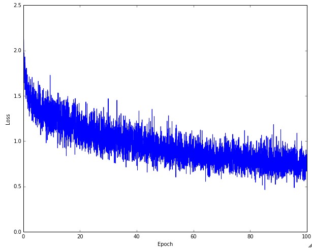
The amount of “wiggle” in the loss is related to the batch size. When the batch size is 1, the wiggle will be relatively high. When the batch size is the full dataset, the wiggle will be minimal because every gradient update should be improving the loss function monotonically (unless the learning rate is set too high).
Some people prefer to plot their loss functions in the log domain. Since learning progress generally takes an exponential form shape, the plot appears as a slightly more interpretable straight line, rather than a hockey stick. Additionally, if multiple cross-validated models are plotted on the same loss graph, the differences between them become more apparent.
Sometimes loss functions can look funny lossfunctions.tumblr.com.
Train/Val accuracy
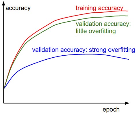
The second important quantity to track while training a classifier is the validation/training accuracy. This plot can give you valuable insights into the amount of overfitting in your model:
Ratio of weights:updates
The last quantity you might want to track is the ratio of the update magnitudes to the value magnitudes. Note: updates, not the raw gradients (e.g. in vanilla sgd this would be the gradient multiplied by the learning rate). You might want to evaluate and track this ratio for every set of parameters independently. A rough heuristic is that this ratio should be somewhere around 1e-3. If it is lower than this then the learning rate might be too low. If it is higher then the learning rate is likely too high. Here is a specific example:
# assume parameter vector W and its gradient vector dW
param_scale = np.linalg.norm(W.ravel())
update = -learning_rate*dW # simple SGD update
update_scale = np.linalg.norm(update.ravel())
W += update # the actual update
print update_scale / param_scale # want ~1e-3
Instead of tracking the min or the max, some people prefer to compute and track the norm of the gradients and their updates instead. These metrics are usually correlated and often give approximately the same results.
Activation / Gradient distributions per layer
An incorrect initialization can slow down or even completely stall the learning process. Luckily, this issue can be diagnosed relatively easily. One way to do so is to plot activation/gradient histograms for all layers of the network. Intuitively, it is not a good sign to see any strange distributions - e.g. with tanh neurons we would like to see a distribution of neuron activations between the full range of [-1,1], instead of seeing all neurons outputting zero, or all neurons being completely saturated at either -1 or 1.
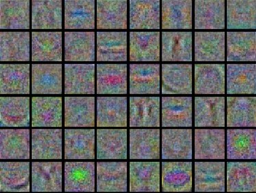
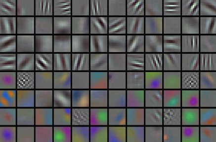
First-layer Visualizations
Lastly, when one is working with image pixels it can be helpful and satisfying to plot the first-layer features visually:
Parameter updates
Once the analytic gradient is computed with backpropagation, the gradients are used to perform a parameter update. There are several approaches for performing the update, which we discuss next.
We note that optimization for deep networks is currently a very active area of research. In this section we highlight some established and common techniques you may see in practice, briefly describe their intuition, but leave a detailed analysis outside of the scope of the class. We provide some further pointers for an interested reader.
SGD and bells and whistles
Vanilla update. The simplest form of update is to change the parameters along the negative gradient direction (since the gradient indicates the direction of increase, but we usually wish to minimize a loss function). Assuming a vector of parameters x and the gradient dx, the simplest update has the form:
# Vanilla update
x += - learning_rate * dx
where learning_rate is a hyperparameter - a fixed constant. When evaluated on the full dataset, and when the learning rate is low enough, this is guaranteed to make non-negative progress on the loss function.
Momentum update is another approach that almost always enjoys better converge rates on deep networks. This update can be motivated from a physical perspective of the optimization problem. In particular, the loss can be interpreted as the height of a hilly terrain (and therefore also to the potential energy since \(U = mgh\) and therefore \( U \propto h \) ). Initializing the parameters with random numbers is equivalent to setting a particle with zero initial velocity at some location. The optimization process can then be seen as equivalent to the process of simulating the parameter vector (i.e. a particle) as rolling on the landscape.
Since the force on the particle is related to the gradient of potential energy (i.e. \(F = - \nabla U \) ), the force felt by the particle is precisely the (negative) gradient of the loss function. Moreover, \(F = ma \) so the (negative) gradient is in this view proportional to the acceleration of the particle. Note that this is different from the SGD update shown above, where the gradient directly integrates the position. Instead, the physics view suggests an update in which the gradient only directly influences the velocity, which in turn has an effect on the position:
# Momentum update
v = mu * v - learning_rate * dx # integrate velocity
x += v # integrate position
Here we see an introduction of a v variable that is initialized at zero, and an additional hyperparameter (mu). As an unfortunate misnomer, this variable is in optimization referred to as momentum (its typical value is about 0.9), but its physical meaning is more consistent with the coefficient of friction. Effectively, this variable damps the velocity and reduces the kinetic energy of the system, or otherwise the particle would never come to a stop at the bottom of a hill. When cross-validated, this parameter is usually set to values such as [0.5, 0.9, 0.95, 0.99]. Similar to annealing schedules for learning rates (discussed later, below), optimization can sometimes benefit a little from momentum schedules, where the momentum is increased in later stages of learning. A typical setting is to start with momentum of about 0.5 and anneal it to 0.99 or so over multiple epochs.
With Momentum update, the parameter vector will build up velocity in any direction that has consistent gradient.
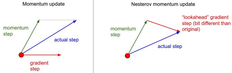
Nesterov Momentum is a slightly different version of the momentum update that has recently been gaining popularity. It enjoys stronger theoretical converge guarantees for convex functions and in practice it also consistenly works slightly better than standard momentum.
The core idea behind Nesterov momentum is that when the current parameter vector is at some position x, then looking at the momentum update above, we know that the momentum term alone (i.e. ignoring the second term with the gradient) is about to nudge the parameter vector by mu * v. Therefore, if we are about to compute the gradient, we can treat the future approximate position x + mu * v as a “lookahead” - this is a point in the vicinity of where we are soon going to end up. Hence, it makes sense to compute the gradient at x + mu * v instead of at the “old/stale” position x.
That is, in a slightly awkward notation, we would like to do the following:
x_ahead = x + mu * v
# evaluate dx_ahead (the gradient at x_ahead instead of at x)
v = mu * v - learning_rate * dx_ahead
x += v
However, in practice people prefer to express the update to look as similar to vanilla SGD or to the previous momentum update as possible. This is possible to achieve by manipulating the update above with a variable transform x_ahead = x + mu * v, and then expressing the update in terms of x_ahead instead of x. That is, the parameter vector we are actually storing is always the ahead version. The equations in terms of x_ahead (but renaming it back to x) then become:
v_prev = v # back this up
v = mu * v - learning_rate * dx # velocity update stays the same
x += -mu * v_prev + (1 + mu) * v # position update changes form
We recommend this further reading to understand the source of these equations and the mathematical formulation of Nesterov’s Accelerated Momentum (NAG):
- Advances in optimizing Recurrent Networks by Yoshua Bengio, Section 3.5.
- Ilya Sutskever’s thesis (pdf) contains a longer exposition of the topic in section 7.2
Annealing the learning rate
In training deep networks, it is usually helpful to anneal the learning rate over time. Good intuition to have in mind is that with a high learning rate, the system contains too much kinetic energy and the parameter vector bounces around chaotically, unable to settle down into deeper, but narrower parts of the loss function. Knowing when to decay the learning rate can be tricky: Decay it slowly and you’ll be wasting computation bouncing around chaotically with little improvement for a long time. But decay it too aggressively and the system will cool too quickly, unable to reach the best position it can. There are three common types of implementing the learning rate decay:
- Step decay: Reduce the learning rate by some factor every few epochs. Typical values might be reducing the learning rate by a half every 5 epochs, or by 0.1 every 20 epochs. These numbers depend heavily on the type of problem and the model. One heuristic you may see in practice is to watch the validation error while training with a fixed learning rate, and reduce the learning rate by a constant (e.g. 0.5) whenever the validation error stops improving.
- Exponential decay. has the mathematical form \(\alpha = \alpha_0 e^{-k t}\), where \(\alpha_0, k\) are hyperparameters and \(t\) is the iteration number (but you can also use units of epochs).
- 1/t decay has the mathematical form \(\alpha = \alpha_0 / (1 + k t )\) where \(a_0, k\) are hyperparameters and \(t\) is the iteration number.
In practice, we find that the step decay is slightly preferable because the hyperparameters it involves (the fraction of decay and the step timings in units of epochs) are more interpretable than the hyperparameter \(k\). Lastly, if you can afford the computational budget, err on the side of slower decay and train for a longer time.
Second order methods
A second, popular group of methods for optimization in context of deep learning is based on Newton’s method, which iterates the following update:
\[x \leftarrow x - [H f(x)]^{-1} \nabla f(x)\]Here, \(H f(x)\) is the Hessian matrix, which is a square matrix of second-order partial derivatives of the function. The term \(\nabla f(x)\) is the gradient vector, as seen in Gradient Descent. Intuitively, the Hessian describes the local curvature of the loss function, which allows us to perform a more efficient update. In particular, multiplying by the inverse Hessian leads the optimization to take more aggressive steps in directions of shallow curvature and shorter steps in directions of steep curvature. Note, crucially, the absence of any learning rate hyperparameters in the update formula, which the proponents of these methods cite this as a large advantage over first-order methods.
However, the update above is impractical for most deep learning applications because computing (and inverting) the Hessian in its explicit form is a very costly process in both space and time. For instance, a Neural Network with one million parameters would have a Hessian matrix of size [1,000,000 x 1,000,000], occupying approximately 3725 gigabytes of RAM. Hence, a large variety of quasi-Newton methods have been developed that seek to approximate the inverse Hessian. Among these, the most popular is L-BFGS, which uses the information in the gradients over time to form the approximation implicitly (i.e. the full matrix is never computed).
However, even after we eliminate the memory concerns, a large downside of a naive application of L-BFGS is that it must be computed over the entire training set, which could contain millions of examples. Unlike mini-batch SGD, getting L-BFGS to work on mini-batches is more tricky and an active area of research.
In practice, it is currently not common to see L-BFGS or similar second-order methods applied to large-scale Deep Learning and Convolutional Neural Networks. Instead, SGD variants based on (Nesterov’s) momentum are more standard because they are simpler and scale more easily.
Additional references:
- Large Scale Distributed Deep Networks is a paper from the Google Brain team, comparing L-BFGS and SGD variants in large-scale distributed optimization.
- SFO algorithm strives to combine the advantages of SGD with advantages of L-BFGS.
Per-parameter adaptive learning rate methods
All previous approaches we’ve discussed so far manipulated the learning rate globally and equally for all parameters. Tuning the learning rates is an expensive process, so much work has gone into devising methods that can adaptively tune the learning rates, and even do so per parameter. Many of these methods may still require other hyperparameter settings, but the argument is that they are well-behaved for a broader range of hyperparameter values than the raw learning rate. In this section we highlight some common adaptive methods you may encounter in practice:
Adagrad is an adaptive learning rate method originally proposed by Duchi et al..
# Assume the gradient dx and parameter vector x
cache += dx**2
x += - learning_rate * dx / (np.sqrt(cache) + eps)
Notice that the variable cache has size equal to the size of the gradient, and keeps track of per-parameter sum of squared gradients. This is then used to normalize the parameter update step, element-wise. Notice that the weights that receive high gradients will have their effective learning rate reduced, while weights that receive small or infrequent updates will have their effective learning rate increased. Amusingly, the square root operation turns out to be very important and without it the algorithm performs much worse. The smoothing term eps (usually set somewhere in range from 1e-4 to 1e-8) avoids division by zero. A downside of Adagrad is that in case of Deep Learning, the monotonic learning rate usually proves too aggressive and stops learning too early.
RMSprop. RMSprop is a very effective, but currently unpublished adaptive learning rate method. Amusingly, everyone who uses this method in their work currently cites slide 29 of Lecture 6 of Geoff Hinton’s Coursera class. The RMSProp update adjusts the Adagrad method in a very simple way in an attempt to reduce its aggressive, monotonically decreasing learning rate. In particular, it uses a moving average of squared gradients instead, giving:
cache = decay_rate * cache + (1 - decay_rate) * dx**2
x += - learning_rate * dx / (np.sqrt(cache) + eps)
Here, decay_rate is a hyperparameter and typical values are [0.9, 0.99, 0.999]. Notice that the x+= update is identical to Adagrad, but the cache variable is a “leaky”. Hence, RMSProp still modulates the learning rate of each weight based on the magnitudes of its gradients, which has a beneficial equalizing effect, but unlike Adagrad the updates do not get monotonically smaller.
Adam. Adam is a recently proposed update that looks a bit like RMSProp with momentum. The (simplified) update looks as follows:
m = beta1*m + (1-beta1)*dx
v = beta2*v + (1-beta2)*(dx**2)
x += - learning_rate * m / (np.sqrt(v) + eps)
Notice that the update looks exactly as RMSProp update, except the “smooth” version of the gradient m is used instead of the raw (and perhaps noisy) gradient vector dx. Recommended values in the paper are eps = 1e-8, beta1 = 0.9, beta2 = 0.999. In practice Adam is currently recommended as the default algorithm to use, and often works slightly better than RMSProp. However, it is often also worth trying SGD+Nesterov Momentum as an alternative. The full Adam update also includes a bias correction mechanism, which compensates for the fact that in the first few time steps the vectors m,v are both initialized and therefore biased at zero, before they fully “warm up”. With the bias correction mechanism, the update looks as follows:
# t is your iteration counter going from 1 to infinity
m = beta1*m + (1-beta1)*dx
mt = m / (1-beta1**t)
v = beta2*v + (1-beta2)*(dx**2)
vt = v / (1-beta2**t)
x += - learning_rate * mt / (np.sqrt(vt) + eps)
Note that the update is now a function of the iteration as well as the other parameters. We refer the reader to the paper for the details, or the course slides where this is expanded on.
Additional References:
- Unit Tests for Stochastic Optimization proposes a series of tests as a standardized benchmark for stochastic optimization.
Hyperparameter optimization
As we’ve seen, training Neural Networks can involve many hyperparameter settings. The most common hyperparameters in context of Neural Networks include:
- the initial learning rate
- learning rate decay schedule (such as the decay constant)
- regularization strength (L2 penalty, dropout strength)
But as we saw, there are many more relatively less sensitive hyperparameters, for example in per-parameter adaptive learning methods, the setting of momentum and its schedule, etc. In this section we describe some additional tips and tricks for performing the hyperparameter search:
Implementation. Larger Neural Networks typically require a long time to train, so performing hyperparameter search can take many days/weeks. It is important to keep this in mind since it influences the design of your code base. One particular design is to have a worker that continuously samples random hyperparameters and performs the optimization. During the training, the worker will keep track of the validation performance after every epoch, and writes a model checkpoint (together with miscellaneous training statistics such as the loss over time) to a file, preferably on a shared file system. It is useful to include the validation performance directly in the filename, so that it is simple to inspect and sort the progress. Then there is a second program which we will call a master, which launches or kills workers across a computing cluster, and may additionally inspect the checkpoints written by workers and plot their training statistics, etc.
Prefer one validation fold to cross-validation. In most cases a single validation set of respectable size substantially simplifies the code base, without the need for cross-validation with multiple folds. You’ll hear people say they “cross-validated” a parameter, but many times it is assumed that they still only used a single validation set.
Hyperparameter ranges. Search for hyperparameters on log scale. For example, a typical sampling of the learning rate would look as follows: learning_rate = 10 ** uniform(-6, 1). That is, we are generating a random number from a uniform distribution, but then raising it to the power of 10. The same strategy should be used for the regularization strength. Intuitively, this is because learning rate and regularization strength have multiplicative effects on the training dynamics. For example, a fixed change of adding 0.01 to a learning rate has huge effects on the dynamics if the learning rate is 0.001, but nearly no effect if the learning rate when it is 10. This is because the learning rate multiplies the computed gradient in the update. Therefore, it is much more natural to consider a range of learning rate multiplied or divided by some value, than a range of learning rate added or subtracted to by some value. Some parameters (e.g. dropout) are instead usually searched in the original scale (e.g. dropout = uniform(0,1)).
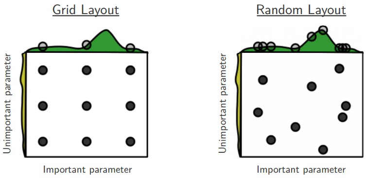
Prefer random search to grid search. As argued by Bergstra and Bengio in Random Search for Hyper-Parameter Optimization, “randomly chosen trials are more efficient for hyper-parameter optimization than trials on a grid”. As it turns out, this is also usually easier to implement.
Careful with best values on border. Sometimes it can happen that you’re searching for a hyperparameter (e.g. learning rate) in a bad range. For example, suppose we use learning_rate = 10 ** uniform(-6, 1). Once we receive the results, it is important to double check that the final learning rate is not at the edge of this interval, or otherwise you may be missing more optimal hyperparameter setting beyond the interval.
Stage your search from coarse to fine. In practice, it can be helpful to first search in coarse ranges (e.g. 10 ** [-6, 1]), and then depending on where the best results are turning up, narrow the range. Also, it can be helpful to perform the initial coarse search while only training for 1 epoch or even less, because many hyperparameter settings can lead the model to not learn at all, or immediately explode with infinite cost. The second stage could then perform a narrower search with 5 epochs, and the last stage could perform a detailed search in the final range for many more epochs (for example).
Bayesian Hyperparameter Optimization is a whole area of research devoted to coming up with algorithms that try to more efficiently navigate the space of hyperparameters. The core idea is to appropriately balance the exploration - exploitation trade-off when querying the performance at different hyperparameters. Multiple libraries have been developed based on these models as well, among some of the better known ones are Spearmint, SMAC, and Hyperopt. However, in practical settings with ConvNets it is still relatively difficult to beat random search in a carefully-chosen intervals. See some additional from-the-trenches discussion here.
Evaluation
Model Ensembles
In practice, one reliable approach to improving the performance of Neural Networks by a few percent is to train multiple independent models, and at test time average their predictions. As the number of models in the ensemble increases, the performance typically monotonically improves (though with diminishing returns). Moreover, the improvements are more dramatic with higher model variety in the ensemble. There are a few approaches to forming an ensemble:
- Same model, different initializations. Use cross-validation to determine the best hyperparameters, then train multiple models with the best set of hyperparameters but with different random initialization. The danger with this approach is that the variety is only due to initialization.
- Top models discovered during cross-validation. Use cross-validation to determine the best hyperparameters, then pick the top few (e.g. 10) models to form the ensemble. This improves the variety of the ensemble but has the danger of including suboptimal models. In practice, this can be easier to perform since it doesn’t require additional retraining of models after cross-validation
- Different checkpoints of a single model. If training is very expensive, some people have had limited success in taking different checkpoints of a single network over time (for example after every epoch) and using those to form an ensemble. Clearly, this suffers from some lack of variety, but can still work reasonably well in practice. The advantage of this approach is that is very cheap.
- Running average of parameters during training. Related to the last point, a cheap way of almost always getting an extra percent or two of performance is to maintain a second copy of the network’s weights in memory that maintains an exponentially decaying sum of previous weights during training. This way you’re averaging the state of the network over last several iterations. You will find that this “smoothed” version of the weights over last few steps almost always achieves better validation error. The rough intuition to have in mind is that the objective is bowl-shaped and your network is jumping around the mode, so the average has a higher chance of being somewhere nearer the mode.
One disadvantage of model ensembles is that they take longer to evaluate on test example. An interested reader may find the recent work from Geoff Hinton on “Dark Knowledge” inspiring, where the idea is to “distill” a good ensemble back to a single model by incorporating the ensemble log likelihoods into a modified objective.
Summary
To train a Neural Network:
- Gradient check your implementation with a small batch of data and be aware of the pitfalls.
- As a sanity check, make sure your initial loss is reasonable, and that you can achieve 100% training accuracy on a very small portion of the data
- During training, monitor the loss, the training/validation accuracy, and if you’re feeling fancier, the magnitude of updates in relation to parameter values (it should be ~1e-3), and when dealing with ConvNets, the first-layer weights.
- The two recommended updates to use are either SGD+Nesterov Momentum or Adam.
- Decay your learning rate over the period of the training. For example, halve the learning rate after a fixed number of epochs, or whenever the validation accuracy tops off.
- Search for good hyperparameters with random search (not grid search). Stage your search from coarse (wide hyperparameter ranges, training only for 1-5 epochs), to fine (narrower rangers, training for many more epochs)
- Form model ensembles for extra performance
Additional References
- SGD tips and tricks from Leon Bottou
- Efficient BackProp (pdf) from Yann LeCun
- Practical Recommendations for Gradient-Based Training of Deep Architectures from Yoshua Bengio